Embedded software developers operate in a perfect digital environment but must interact with the imperfect analog real world. To do this it's essential to know how to perform calibration of inputs and sensors.
A few years back, a Barr Group client was developing a piece of physical therapy equipment that was to provide a variable number of pounds of force feedback to a human operator. To support the complete range of possible force settings with a given worst-case accuracy, the product was correctly designed around a microcontroller. The embedded software that ran on this microcontroller was principally responsible for regulating the voltage going to a brake such that the brake's calipers would "slip" precisely at the selected force. In other words, the human operator must push or pull against the shaft with at least the selected amount of force in order to make the shaft move. But the problem did not turn out to be as easy as it at first appeared.
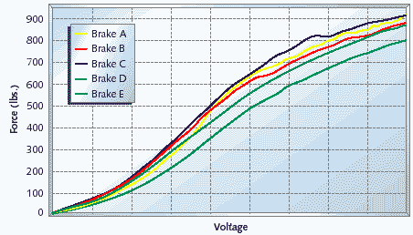
What made this problem so difficult was that each brake performed differently in actual use. It turns out that there's no one equation that says: to achieve x pounds of force, apply v = f(x) volts. (The input to the brake was actually a PWM signal and the important characteristic was current; I'm using voltage to make the discussion simpler.) Figure 1 contains five S-shaped curves. Each of these curves is the measured response of a particular brake. And, as if the differences between brakes were not enough to deal with, the curve for each particular brake is affected by its age (as the contacting surfaces wear), temperature, and even the velocity of the force applied against it. (All of these are factors that alter the amount of friction between the surfaces.)
Perhaps the first and most obvious step to take is to create a feedback loop in the system. It's clear that simply setting the voltage on the brake and forgetting it is not going to be good enough. As you can see from Figure 1, the difference in force output for a given voltage between brakes can be extremely large. Some of the brake curves even cross, indicating that individual brakes are not simply stronger or weaker than the average.

Figure 1. Measured brake curves
By adding sensors that can read the applied force and the shaft's position, it is possible to make continuous adjustments to the brake voltage as the user is in the process of pushing or pulling on the shaft. If the shaft is moving (its position is changing) and the force on the shaft is too small, the brake voltage must be increased. If the force is too high, the voltage must be decreased. By "closing" toward the desired force like this, it's possible to achieve and maintain that force throughout each repetition of the exercise.
One problem with such a closed-loop approach is that it takes time to achieve the desired results. If you close too quickly, you'll continually overshoot and undershoot the desired force. So you must only make one small change in the voltage in a given time period, then wait for the brake to respond before making the next change. In our case, we found the ideal period to be right around 50ms. At that rate of closure, you can be relatively certain of achieving the desired force without much overshoot, and maintaining it without too much fluctuation.
However, if you start out with an initial force that is so far from the desired force that it takes more than about half a second (500ms) to reach it, a human can generally feel the change in resistance. This seems to be true whether the incorrect initial force is above or below the desired force. So more than 10 increment or decrement operations had to be avoided at all costs. And the only way to achieve that was to make a fairly accurate initial "guess" about what the brake voltage should be for a given force. To get that kind of accuracy, we had to calibrate each brake's S-curve when it was installed. And, because of the more subtle brake-specific factors mentioned previously, each brake must be periodically recalibrated in the field.
Linear simplicity
Before we can talk about calibrating the brakes, however, we must first talk about the force sensors. Each force sensor must also be calibrated. Consider the example of a force sensor that always reads 10% below the actual force applied. The user will have to apply significantly more force (11.1% more, to be exact) than he or she expected. If you might be tempted to consider that a tolerable worst-case error, remember that it is possible the human user could injure (or, more likely, reinjure) a muscle in the process of completing an exercise on such a strongly biased machine.
Fortunately, calibrating the force sensors is not terribly complicated. It turns out that these devices can only really be biased in one of three ways. (This from the manufacturer, of course.) First, they may have a non-zero reading even when no force is applied to them. We'll call this the sensor's zero offset. Second and third, the sensors may have a linear bias unique to forces applied in each direction. We'll call these the left and right gain factors.
The zero offset is easy to determine and correct for. You need only read the force reported by the sensor when no force is applied. That value is the zero offset for that particular sensor. To correct for it, simply subtract the zero offset from every future force reading. For example, if you determine that the zero offset is 5 lbs. and your next "raw" reading is 15 lbs., you'd compute the actual force on the shaft to be 10 lbs.
Once the zero offset, if any, has been subtracted out, determining the left and right gain factors is possible. The terms left and right are subjective, of course, but the general idea is that the sensor has one linear bias when forces are applied in one direction and a different linear bias when forces are applied in the opposite direction. The fact that these biases are linear simply means that the percentage error is the same, regardless of the actual force applied. So, for example, a sensor with a -10% bias would read 90 lbs. when 100 lbs. is applied and 180 lbs. when 200 lbs. is applied. It is, therefore, sufficient to take one calibration reading in each direction.
To determine the left and right gain factors, you might simply hang a 100-lb. weight from the shaft, first applying that force in one direction then the other. By comparing the actual readings to the expected readings in each direction, you can compute the sensor's left and right gain factors. By dividing all future readings by the gain factor in the given direction, you can eliminate these biases from the sensor. The result is an accurate measure of force that can be compared across different machines and form the basis for calibration of the brakes. Figure 2 Nominal break curve Figure 3 A polynomial approximation of the nominal state
Polynomial insanity
Calibrating a brake is much harder than calibrating a force sensor, for one important reason: each brake's S-curve is non-linear. You can't simply take one reading and compute a gain factor from it. This was possible for the sensors only because their error was a fixed percentage of their input value. The brakes, on the other hand, can diverge wildly from one another (and even from themselves, over time), so that there's really no such thing as a typical brake.
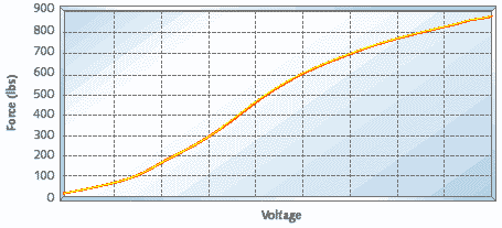
Despite the fact that there is no typical brake, we've still got to define one. After all, you need a starting point even just to perform a calibration. So we began by measuring the relationship between input voltage and output force for five randomly selected brakes. The results of these measurements were the five data sets shown in Figure 1. We then averaged the five forces resulting from each tested voltage setting to produce the nominal brake curve shown in Figure 2.

Figure 2. Nominal brake curve
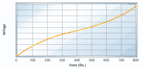
The only problem with the curve in Figure 2 is that it represents the inverse of the relationship the software needs to compute at run-time. The necessary relationship measures voltage as a function of desired force, telling the microcontroller how much voltage it should apply to the brake to achieve a particular desired force. Figure 3 shows the same nominal brake data, flipped on its axes and approximated as the third-order polynomial:
v = Ax3 + Bx2 + Cx + D (Equation 1)
where A, B, C, and D are floating-point coefficients. Jack Crenshaw has recently been looking to tackle a similar sort of problem in the pages of his column--that is, run-time calibration of a device with a polynomial response curve. However, his approach seems to be to actually determine new coefficients (A, B, C, and D) at run time, thus performing a complicated set of computations on the embedded processor. That sort of approach simply wasn't practical in this particular system.

Figure 3. A polynomial approximation of the nominal brake
What made more sense was for us was to try to "tweak" the nominal curve to make it a better fit for each particular brake. This was partly because we didn't have the computational resources to spare (it was only an 8-bit processor with a couple hundred bytes of RAM, after all) and partly because we were able to "close" to the desired force pretty quickly anyway. All we really needed to accomplish through calibration was to bring the curve within about 10 voltage increments or decrements of the optimal value, along as much of the curve as possible. In truth, given all of the other factors affecting the brake performance, we could never really hope for anything better. The actual brake curve will change, for example, as soon as the surface of the brake pads heats up (even after just a few reps).
Here's how tweaking the curve might work in practice. Given a particular force setting, x, the nominal voltage, v, would be computed according to the polynomial in Equation 1. We would then apply a "tweak factor" that is also a function of the force. In other words, we'd apply a "local" tweak factor that is applicable only at or very near x lbs. Multiplying the nominal voltage by the tweak factor, we'd get a new voltage, v', and apply that to the brake. The result, we hope, will be a force within 10 voltage increments or decrements of the optimal voltage. If it is, we've done good enough.
This, of course, begs the question of how to determine those "tweak factors."
Tweaking
The key to tweaking is the number of data points. If we had the luxury of setting the brake to every possible voltage and measuring the resulting forces, it is clear that we could produce an exact tweak factor for every point along the curve. For any given force, the actual brake curve may be above, on top of, or below the nominal curve. (Above means a higher voltage is needed to achieve that force on this particular brake at this particular time, below means a lower voltage.) If it's above the nominal curve, the tweak factor would be a number greater than 1.0; if it's below, the tweak factor would be less than 1.0; and if the actual and nominal brakes concur at that force, the tweak factor would be exactly 1.0.
Unfortunately, measuring the force produced by every brake at every possible voltage is not realistic. (It was hard enough doing that once for each of the five representative brakes.) Since calibration must be done frequently and it is often the owner of the machine who will do it, it is necessary that the number of data points be significantly reduced.
At each calibration data point, a specific force (x1) is requested, the microcontroller computes the nominal voltage for that force (v1), the nominal voltage is applied to the brake, and the force produced is recorded. Interestingly, the processor now knows exactly what voltage to input to achieve the force that resulted-though it still doesn't know how to produce the requested force. In other words, if the next force requested were the one we had just produced (call it x2) it would be very easy to "tweak" the nominal curve at that point, by simply multiplying the nominal voltage by the ratio of the two voltages (v1/v2). This ratio is the tweak factor at force x2.
By taking a number of these measurements and recording the ordered pairs (x2, v1/v2) in a table, we gain the ability to produce perfect results at those specific requested forces. To extend these results to include other forces, we simply "draw" line segments between each known data point. In other words, we weight the two closest "precise" tweak factors to achieve estimated tweak factors for any force in between.
typedef struct
{
    uint16_t force;
    double   ratio;

} CalPoint;

CalPoint aCalPoints[NUM_CAL_POINTS];

uint16_t
adjustVoltage(uint16_t force, uint16_t vNominal)
{
    int     i;
    double  scaleFactor;


   /*
    * Find the relevant calibration range.
    */
   for (i = 1; i < NUM_CAL_POINTS && aCalPoints[i].force < force; i++);

   /*
    * Compute the weighted scale factor.
    */
   scaleFactor = ((aCalPoints[i].force - force) * aCalPoints[i-1].ratio
               + (force - aCalPoints[i-1].force) * aCalPoints[i].ratio)
               / (aCalPoints[i].force - aCalPoints[i-1].force);

   /*
    * Adjust the voltage.
    */
   return (vNominal * scaleFactor);

}  /* adjustVoltage() */
Listing 1. A function that uses the calibration data
Listing 1 contains a function, adjustVoltage(), that performs the voltage scaling mathematics. The data structure is an array of calibration data points. Each CalPoint consists of a force (x2) and a ratio (v1/v2) that was observed when the force x1 was most recently tested on this brake. These calibration points are assumed to be ordered in the array from the smallest force to the largest. In addition, the function assumes that the array begins with a calibration point at force 0 and ends with a calibration point at MAX_FORCE. (We found that the ratios associated with these two points should be set to 1.0 and the same as the highest actual calibration point available, respectively.)
In effect, we multiply the nominal curve by a connected set of line segments. The more data points you have, the shorter the line segments will be, and, therefore, the more precise the resulting calibration. This is a really practical way to calibrate a complex device quickly. In our specific case, we were able to take just five measurements during brake calibration and to achieve impressive results.
I haven't found much literature about doing this sort of run-time calibration, so I wonder how others have accomplished similar tasks in their embedded systems. If you have a war story or a favorite reference on the subject, please share in a comment below.
This column was published in the May 2000 issue of Embedded Systems Programming. If you wish to cite the article in your own work, you may find the following MLA-style information helpful:
Barr, Michael. "Hold Everything," Embedded Systems Programming, May 2000 , pp. 53-59.


